Hypothesis Testing And Goodness of Fit
Contents
Hypothesis Testing And Goodness of Fit#
The \(\chi^2\) distribution describes how the sum of the square of independent standard normal random variables are distributed, ie \(Q\) the sum of the squares
if
and,
This is useful in error analysis as when we have a data point with an associated error, it can be treated as a randomly distributed normal variable, and the square residual, can be seen as a squared random variable. The residual can be standardized by dividing by the square of the error. Thus, we have a probability distribution that describes the sum of all the squared errors. This can then be used as a ‘goodness of fit metric’. On top of such a metric, hypothesis testing introduces a framework for deciding weather to accept or reject a model dependent on the \(\chi^2\) value.
Hypothesis testing and \(\chi^2\) statistics tests quantify the validity and ‘goodness of fit’, respectively. Again a thorough treatment of the \(\chi^2\) statistic is presented in chapters 5 and 8 of ‘Measurements and Their Uncertainties’[HH10]. The statistic is defined for a model,\(y'\), and data,\(y\),! as,
If each value in the residual sum is treated as an independent random variable. Then the sum of the values is distributed according to,
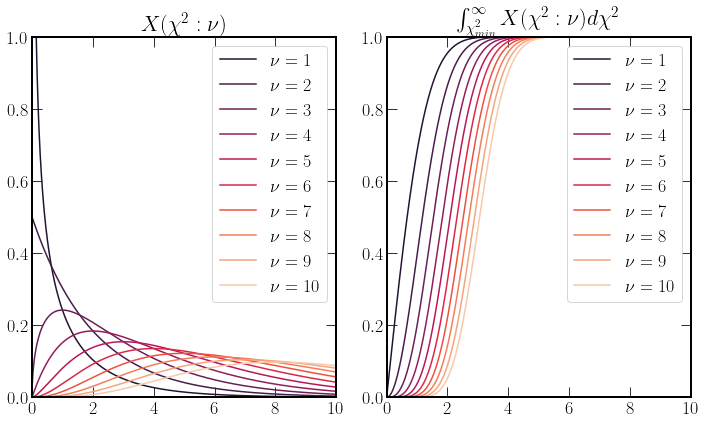
Both the PDF(probability density function) and CDF(cumulative density function) are plotted below left and right, respectively, for \(\nu\) up to ten. The degrees of freedom, \(\nu = N - m\), where N and m are the numbers of data points and parameters, respectively.
The CDF quantifies the probability that the residuals are larger, for a specific model with a \(\chi^2\), \(P(\chi^2 \geq \chi^2_{min};\nu)\). A good fit is indicated by a value close to one. Bearing in mind that the \(\chi^2\) considers the size of the errors present. A small value for \(P(\chi^2 \geq \chi^2_{min};\nu)\) can be an indication of overly large error.
The test is based on the ratio of the residuals to their expectations and how one would expect them distributed. The expectation value for the PDF is \(\nu\) and so the reduced statistic
Should be close to one for a good fit.
x = np.linspace(0, 10, 1000)
# Plotting
fig, ax = plt.subplots(1, 2, figsize=(10, 6))
for spt in ax:
    spt.set_prop_cycle(color=sns.color_palette("rocket", 10))
for i in range(10):
    pdf = stats.chi2.pdf(x, 1 + i)
    cdf = stats.chi.sf(x, 1 + i)
    ax[0].plot(x, pdf, label=r"$\nu$" + f" = {i+1}")
    ax[1].plot(x, 1 - cdf, label=r"$\nu$" + f" = {i+1}")
for spt in ax:
    spt.legend()
    spt.set_ylim(0, 1)
    spt.set_xlim(0, 10)
ax[0].set_title(r"$ X(\chi^2:\nu) $")
ax[1].set_title(r"$ \int_{\chi^2_{min}}^\infty X(\chi^2:\nu) d \chi^2 $");

Hypothesis Testing#
Hypothesis testing provides a systematic framework for deciding if a model fits set of data. The process for the Pearson \(\chi^2\) test is as follows. Given a null hypothesis \(\mathcal{H}_0\), in which the model describes the data. Additionally, define an alternate hypothesis \(\mathcal{H}_1\)
Determine the \(\chi^2\) value for the data
Determine \(\nu\)
Select a confidence level and calculate \(\chi^2_{crit}\)
Compare The Value of \(\chi^2_{min}\) with \(\chi^2_{crit}\)
Reject \(\mathcal{H}_0\) if \(\chi^2_{min} \geq \chi^2_{crit}\), in favour of \(\mathcal{H}_1\)
Hypothesis testing provides a framework for quantatively assessing wheather a new model should be produced.
Implementing \(\chi^2\) testing in \(\text{CO}_2\) data#
Below, behind the toggles are a set of functions used to fit the data and calculate \(\chi^2\).
"""
In this code block, first two different polynomials are defined.
The scipy curve fit package is used to fit the datapoints to the values.
Then the residuals from these curves are used to evaluate the curves chi^2.

The rs prefix is used to indicate a residual variable
The y prefix indicates the values calculated  by the curve fit.

The ml prefix is for mauna  loa data.
The global prefix is for the global data.
"""
def p3(x, a_0, a_1, a_2, a_3):
    return a_0 + a_1 * x + a_2 * x**2 + a_3 * x**3


def p1(x, a_0, a_1):
    return a_0 + a_1 * x


# Fit Coefs
##Unweighted Least Squares Global
p1_global_fit, p1_global_error = scipy.optimize.curve_fit(
    p1, co2_data_global["decimal"], co2_data_global["average"]
)
# chisq
y_p1_global = p1(co2_data_global["decimal"], *p1_global_fit)
rs_global_p1 = y_p1_global - co2_data_global["average"]
chisq_global_p1 = np.sum(
    ((rs_global_p1) / np.mean(co2_data_global["decimal"] ** 2) ** 0.5) ** 2
)
# P3
p3_global_fit, p3_global_error = scipy.optimize.curve_fit(
    p3, co2_data_global["decimal"], co2_data_global["average"]
)
# chisq
y_p3_global = p3(co2_data_global["decimal"], *p3_global_fit)
rs_global_p3 = y_p3_global - co2_data_global["average"]
chisq_global_p3 = np.sum(
    ((rs_global_p3) / np.mean(co2_data_global["decimal"] ** 2) ** 0.5) ** 2
)
# Weighted Least Squares Mauna Loa
p1_ml_fit, p1_ml_error = scipy.optimize.curve_fit(
    p1,
    co2_data_ml["decimal date"],
    co2_data_ml["average"],
    sigma=co2_data_ml["sdev"],
)
y_p1_ml = p1(co2_data_ml["decimal date"], *p1_ml_fit)
rs_ml_p1 = y_p1_ml - co2_data_ml["average"]
chisq_ml_p1 = np.sum(((rs_ml_p1) / co2_data_ml["sdev"]) ** 2)
# P3
p3_ml_fit, p3_ml_error = scipy.optimize.curve_fit(
    p3,
    co2_data_ml["decimal date"],
    co2_data_ml["average"],
    sigma=co2_data_ml["sdev"],
)

y_p3_ml = p3(co2_data_ml["decimal date"], *p3_ml_fit)
rs_ml_p3 = y_p3_ml - co2_data_ml["average"]
chisq_ml_p3 = np.sum(((rs_ml_p3) / co2_data_ml["sdev"]) ** 2)
Calculating \(P(\chi^2 \geq \chi^2_{min};\nu)\)#
"""
Here the scipy package is used to evaluate the probability that the
residuals are not randomly distributed.
This is done using the survival function chi2.sf, which is 1-cdf.
"""
nu_p1_ml = co2_data_ml["average"].shape[0] - len(p1_ml_fit)
nu_p3_ml = co2_data_ml["average"].shape[0] - len(p3_ml_fit)
p_ml_p1 = stats.chi2.sf(chisq_ml_p1, nu_p1_ml)
p_ml_p3 = stats.chi2.sf(chisq_ml_p3, nu_p3_ml)
print(rf"P(\chi^2 \geq \chi^2_{{min}};{nu_p1_ml}) = {p_ml_p1}")
print(rf"P(\chi^2 \geq \chi^2_{{min}};{nu_p3_ml}) = {p_ml_p3}")
P(\chi^2 \geq \chi^2_{min};582) = 0.0
P(\chi^2 \geq \chi^2_{min};580) = 0.0
"""
This plotting section unlike many is rather extensive, because both
plots have residual sections below the actual figure, the implementation
is splot into making the plot shape and populating the plot.
"""

dur_cycle = cycler(
    color=[colours.durham.ink, colours.durham.purple, colours.durham.blue]
)

# Building Subplot list, add axis builds from bottom left
total_fig_height = 2
total_fig_width = 2
fig = plt.figure(figsize=(4.5, 7.5))
fig.set_tight_layout(False)
ax = []
current_fig_bottom = 0
for i in range(4):
    if i % 2 != 0:
        height = total_fig_height / 3

        ax.append(
            fig.add_axes([0, current_fig_bottom, total_fig_width, height])
        )
        current_fig_bottom += height + total_fig_height / 12
    else:
        height = total_fig_height / 8
        ax.append(
            fig.add_axes([0, current_fig_bottom, total_fig_width, height])
        )
        current_fig_bottom += height
# Lists for plotting
# glob
fits_global = [y_p1_global, y_p3_global]
chisq_global = [chisq_global_p1, chisq_global_p3]
rs_glob = [rs_global_p1, rs_global_p3]
glob = zip(fits_global, chisq_global, rs_glob)
# ml
fits_ml = [y_p1_ml, y_p3_ml]
chisq_ml = [chisq_ml_p1, chisq_ml_p3]
rs_ml = [rs_ml_p1, rs_ml_p3]
ml = zip(fits_ml, chisq_ml, rs_ml)
# Plotting
for i, spt in enumerate(ax):
    # spt.text(0.5, 0.5, "ax%d" % (i), va="center", ha="center")
    spt.set_ylabel(r"$\textrm{{CO}}_2$ (ppm)")
    if i % 2 != 0:
        spt.set_prop_cycle(dur_cycle)
    else:
        cp = dur_cycle
        cp = cp[1:]
        spt.set_prop_cycle(cp)
    spt.set_xlim(1980, 2022)
ax[3].plot(
    co2_data_global["decimal"],
    co2_data_global["average"],
    linestyle="",
    marker=".",
)
ax[1].errorbar(
    co2_data_ml["decimal date"],
    co2_data_ml["average"],
    co2_data_ml["sdev"],
    linestyle="",
    capsize=1,
)
for i, (
    (glob_f, glob_chi, residual_global),
    (ml_f, ml_chi, residual_ml),
) in enumerate(zip(glob, ml)):
    # ml plot
    ax[1].plot(
        co2_data_ml["decimal date"],
        ml_f,
        label=f"P{2*i + 1}: " + r"$\chi^2_{min}$ = " + f"{ml_chi:.3}",
    )
    ax[0].errorbar(
        co2_data_ml["decimal date"],
        residual_ml,
        co2_data_ml["sdev"],
        linestyle="",
        capsize=2,
    )
    # global
    ax[3].plot(
        co2_data_global["decimal"],
        glob_f,
        label=f"P{2*i + 1}: " + r"$\chi^2_{min}$ = " + f"{glob_chi:.3}",
    )
    ax[2].plot(
        co2_data_global["decimal"],
        residual_global,
        marker="+",
        linestyle="",
    )

ax[1].legend()
ax[3].legend()
ax[0].set_xlabel("Years")
ax[2].set_xlabel("Years")
ax[1].set_title("Mauna Loa")
ax[3].set_title("Global Average");

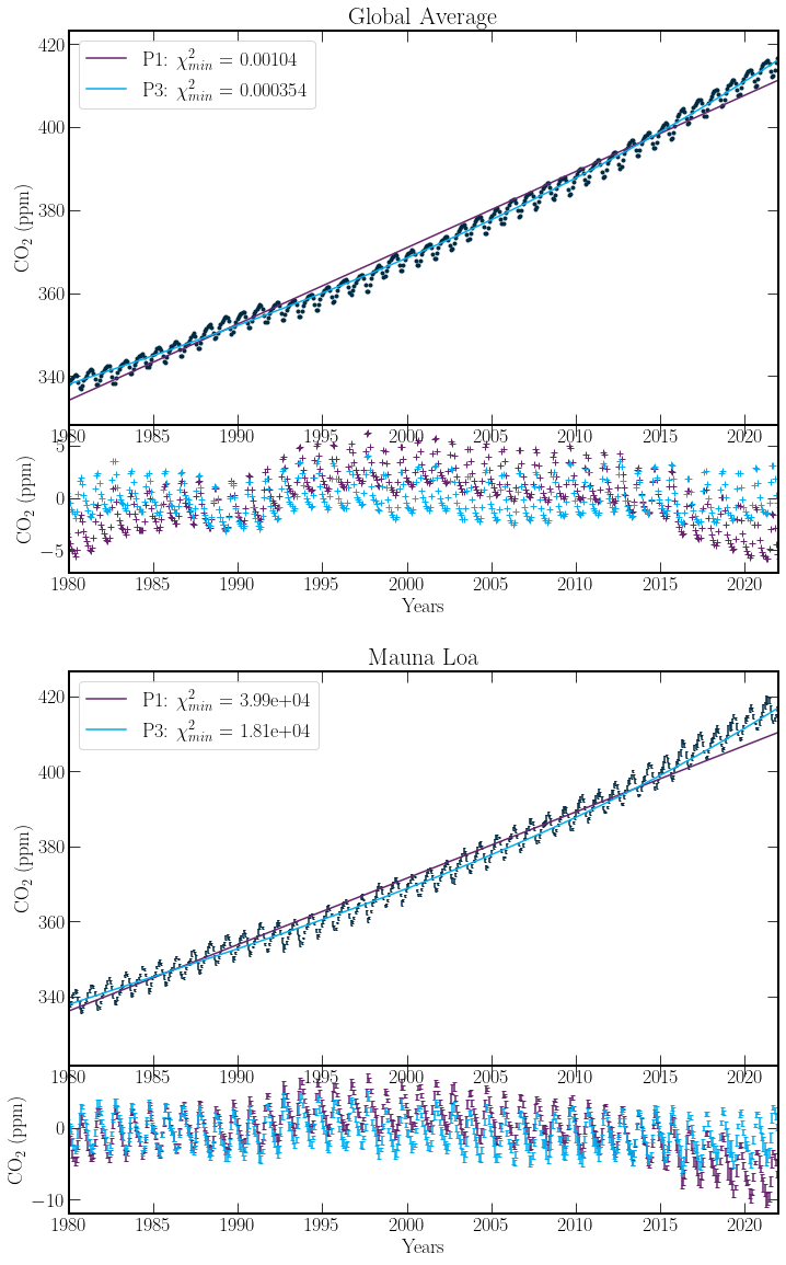
The \(P(\chi^2 \geq \chi^2_{min};\nu) = 0.0\), values are infact expected. On inspection, the error on each measurement is of the order \(0.1\) ppm. However, the magnitude of the residuals regularly is of the order \(1\) ppm. As such, the fit to the Mauna Loa Data should be poor. With climate data of this sort, the measurement of the individual datapoints is very accurate, however due to variance in the systems such as volcanoes, wildfires or other carbon emitters or sinks mean having a trend that fits these across many years is unlikely. Nevertheless, the third order polynomial across both global and Mauna Loa data sets provides much better agreement. This will be the model taken forward.
The residuals also have a regular periodic structure. Fitting the residuals to a function of the form,
Gives periodicity to our function. Discovering the value of the \(\omega\) co-efficients can prove difficult using the current techniques.
Least-squares fitting of \(\sin(x)\) and \(\cos(x)\) can be problematic. The presence of many local minima hinders convergence. To determine the periodicity of the residuals one can use Fourier techniques.
Fourier Transforms#
There are whole texts dedicated to the subtleties of Fourier analysis. For an intuitive picture of how the technique works, this video is excellent.
The 1D Fourier and inverse Fourier transforms are defined as integrals over all real numbers. The precise definition of the transform can vary. However, the general form of transform and its inverse are respectively
Clearly with, the discrete data provided by the residuals, such definitions must be adjusted. Due to problems of this form being common across many disciplines, the Fast Fourier transform(FFT)[CLW69] was developed to perform these calculations efficiently. Additionally, a Discrete Cosine Transform(DCT)[ANR74] can be used because the data is real-valued, and sampled at a constant frequency.
The DCT provides binned results. So our main frequencies generated by the DCT will be limited in precision. Thus The DCT results can be used to provide starting values for the least-squares method.
# Show data is sampled at constant freq
timesteps = co2_data_ml["decimal date"] - np.roll(
    co2_data_ml["decimal date"], -1
)
timesteps = timesteps[:1]
const_freq = np.isclose(timesteps, timesteps.iloc[0])
print("Constant frequncy of CO_2 measurment:", const_freq[0])
print(f"Timestep:{abs(timesteps.iloc[0]):.2}")
Constant frequncy of CO_2 measurment: True
Timestep:0.083
Application of The DCT#
Depending on the application different fomulations of the discrete cosine transform can be used. Here the default type is used, Type-2
This gives a frequency in years of
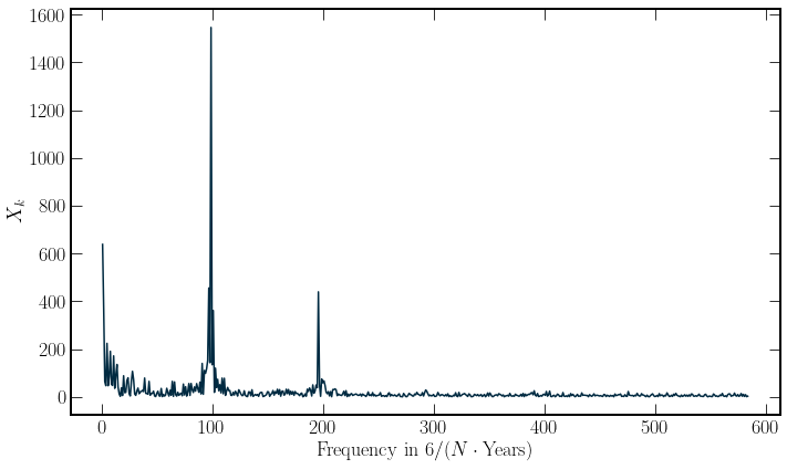
\(\Delta T\) is the time spacing between samples in the time series and \(N\) is the number of entires in the series. For different formulations of the transform the frequency of the bins is calculated from the argument of the cosine being equal to \(2\pi fn\). The output spectra is plotted below.
"""
In this block we use the scipy fft package to evaluate the DCT of the
residuals. This is plotted, to identify the major peaks.
"""

ft_p3_res = fft.dct(np.array(rs_ml_p3))
plt.figure(figsize=(10, 6))
plt.plot(
    range(1, len(ft_p3_res) + 1), abs(ft_p3_res), c=colours.durham.ink
)
plt.xlabel(r"Frequency in $6/(N \cdot \textrm{{Years}})$")
plt.ylabel("$X_k$");

The result of the DCT is reassuring in that the most significant frequency component is the yearly component. However, the prominent peak of the first bin corresponds to the parabolic shape of the mean residuals and so should not be used. Additionally a Bi annual componenet is also seen. These two peaks are taken

