Implementation of the Three SRES Approximation Models
Contents
Implementation of the Three SRES Approximation Models#
The three approximate SRES scenarios chosen will be used to develop Bayesian temperature change prediction. The model of global temperatures \(T\) as a function of \(\textrm{CO}_2 (C)\) is,
\(S\) describes the sensitivity of the global temperature to doubling in \(\textrm{CO}_2\) concentration. This parameter has proved challenging to estimate given the complexity of the systems influencing global temperature Change. A PDF of \(S\), \(P(S)\) was produced by Sherwood et al.[SWA+20] and will be used for our future temperature predictions and approximations of the SRES scenarios. The PDF of temperature change can be written as
Note
In this model Radiative Forcing is neglected, this id the phenomenon which describes the global flux inbalance. Where more enenrgy is being let out than let in. This is a key part of the global temperature rise equation as this is not a constant factor when global temperatures rise. For a more thourough predictive with radiative forcing see Sherwood2022[SGS22].
The quantity \(P(\Delta T|S)\) can be calculated using our simple climate model eq.(15).
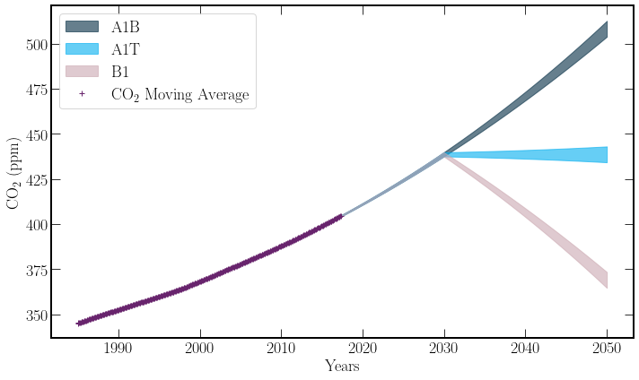
The model will have three separate cases. As discussed before they are as follows:
A1B) Continued growth in emission Rates.
A1T) Net-zero by 2030, no further reductions.
B1) Net-zero by 2030, and then reducing total atmospheric carbon at the same rate it is currently produced.
import pandas as pd
import numpy as np
import matplotlib.pyplot as plt
from dur_utils import colours
from scipy.optimize import curve_fit
from scipy.interpolate import LSQUnivariateSpline

plt.style.use("../CDS.mplstyle")
# Loading fits
model_fit = pd.read_csv(
    "../output_files/co2_model_parameters.csv",
    index_col=0,
).squeeze("columns")
model_error = pd.read_csv(
    "../output_files/co2_model_parameters_errors.csv",
    index_col=0,
).squeeze("columns")
# select only polynomials
poly_fit = model_fit[["c", "p_1", "p_2", "p_3"]]
poly_error = model_error[["c", "p_1", "p_2", "p_3"]]
# Loading Moving average Data
path = (
    "http://berkeleyearth.lbl.gov/auto/Global/Complete_TAVG_complete.txt"
)
# Formatting be data
colnames = [
    "year",
    "month",
    "monthly_anomaly",
    "monthly_anomaly_unc",
    "yearly_anomaly",
    "yearly_anomaly_unc",
    "5yearly_anomaly",
    "5yearly_anomaly_unc",
    "10yearly_anomaly",
    "10yearly_anomaly_unc",
    "20yearly_anomaly",
    "20yearly_anomaly_unc",
]
temp_data = pd.read_fwf(path, skiprows=34, names=colnames)
temp_data["dt"] = temp_data["month"] / 12 + temp_data["year"]
# remove be moving averages
temp_data.drop(
    columns=[
        "yearly_anomaly",
        "yearly_anomaly_unc",
        "5yearly_anomaly",
        "5yearly_anomaly_unc",
        "10yearly_anomaly",
        "10yearly_anomaly_unc",
        "20yearly_anomaly",
        "20yearly_anomaly_unc",
    ],
    inplace=True,
)
\(\textrm{CO}_1\) Concentration Models#
In the final partof[Chapter0](…/ Chapter_1 / Final_Model.ipynb), a polynomial model with a trigonometric addition was developed to characterize the Mauna Loa \(\textrm{CO}_1\) concentration, which closely follows the global average trend.Using the model without the trigonometric terms will be the basis for this section.
def simple_climate_model(
    C: pd.DataFrame, S: int, C_0: int, T_0: int
) -> pd.DataFrame:
    """Model fuction for Temperature and CO_2 relationship."""
    # Placeholder till I figure out what I am going to
    return T_0 + np.log2(C / C_0) * S


# Legacy Functions to have remove imput tag
def lb_ub(values, sigma, factor=1):
    lb = values - sigma * factor
    ub = values + sigma * factor
    return lb, ub


# Models
def a1t(x, p_0, p_1, p_2, p_3, translation=0):
    emissions_stop = np.where(x + translation >= 2030)[0]
    f_eval = p_0 + p_1 * x + p_2 * x**2 + p_3 * x**3
    f_eval[emissions_stop[0] :] = f_eval[emissions_stop[0] - 1]
    return f_eval


def B1(x, p_0, p_1, p_2, p_3, translation=0):
    emissions_stop = np.where(x + translation >= 2030)[0]
    f_eval = p_0 + p_1 * x + p_2 * x**2 + p_3 * x**3
    f_neg = (
        2 * f_eval[emissions_stop[0] - 1]
        - p_0
        - (p_1 * x + p_2 * x**2 + p_3 * x**3)
    )
    f_eval[emissions_stop[0] - 1 :] = f_neg[emissions_stop[0] - 1 :]
    return f_eval


def A1M(x, p_0, p_1, p_2, p_3):  # A1M
    return p_0 + p_1 * x + p_2 * x**2 + p_3 * x**3
The Problem with Polynomials#
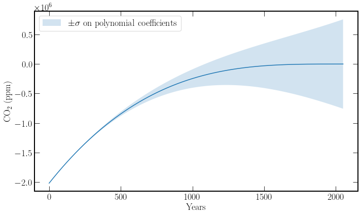
Problems arise when fitting polynomials of order greater than one, minor parameter tweaks to the higher powers’ constants cause large deviations in the value of the function. This can be seen below in the figure, where adjusting the fit parameters by one sigma provides a huge variance in the output of the function. This problem is especially apparent as the data is rather linear, and thus there is a moderate uncertainty on the \(x^2, x^3\) terms.
df = pd.DataFrame(abs(poly_fit / poly_error))
df.columns = ["Fit_Value/Error"]
df
| Fit_Value/Error | |
|---|---|
| c | 4.350885e+15 |
| p_1 | 3.373409e+15 |
| p_2 | 1.193713e+01 |
| p_3 | 1.205885e+01 |
# time = np.linspace(temp_data['dt'].iloc[-1], 2050, 1000)
time = np.linspace(0, 2050, 1000)
lb_coef, ub_coef = lb_ub(poly_fit, poly_error)
plt.figure(figsize=(10, 6))
plt.plot(time, A1M(time, *poly_fit))
plt.fill_between(
    time,
    A1M(time, *lb_coef),
    A1M(time, *ub_coef),
    alpha=0.2,
    label="$\pm \sigma$ on polynomial coefficients",
)
plt.ylabel(r"$\textrm{CO}_2$ (ppm)")
plt.xlabel("Years")
plt.legend(loc="upper left");

To solve this problem, the \(x\) values of the training data, years, can be translated so that they center about zero. Thus the deviations due to small parameter changes are not as large.
Alternatively, a natural spline fit could be used, treating the extrapolation as linear, and thus the range of values inside the \(2 \cdot \sigma\) interval would not diverge as rapidly.
# x values
time = np.linspace(1985, 2050, 1000) - 2000
# Loading CO2 moving averages caluclated previously
co2_ave = pd.read_csv(
    "../output_files/co2_10_moving_average.csv", header=0, index_col=0
)
co2_std = pd.read_csv(
    "../output_files/co2_10_moving_std.csv", header=0, index_col=0
)
co2_mov_fit, co2_mov_cov = curve_fit(
    A1M,
    co2_ave["decimal"] - 2000,
    co2_ave["average"],
    sigma=co2_std["average"],
)
# 2 sigma deviation from fit
co2_mov_error = np.diagonal(co2_mov_cov) ** 0.5
co2_lb_mov, co2_ub_mov = lb_ub(co2_mov_fit, co2_mov_error, factor=2)
sigma = A1M(time, *co2_ub_mov) - A1M(time, *co2_mov_fit)
# Plotting
plt.figure(figsize=(10, 6))
# Models
plt.fill_between(
    time,
    A1M(time, *co2_lb_mov),
    A1M(time, *co2_ub_mov),
    color=colours.durham.ink,
    alpha=0.6,
    label="A1B",
)
plt.fill_between(
    time,
    a1t(time, *co2_mov_fit, translation=2000) - sigma,
    a1t(time, *co2_mov_fit, translation=2000) + sigma,
    color=colours.durham.blue,
    alpha=0.6,
    label="A1T",
)
plt.fill_between(
    time,
    B1(time, *co2_mov_fit, translation=2000) - sigma,
    B1(time, *co2_mov_fit, translation=2000) + sigma,
    color=colours.durham.pink,
    alpha=0.6,
    label="B1",
)
# Data
plt.plot(
    co2_ave["decimal"] - 2000,
    co2_ave["average"],
    linestyle="",
    marker="+",
    color=colours.durham.purple,
    label=r"$\textrm{{CO}}_2$ Moving Average",
)
# Formatting
plt.xticks(range(-10, 60, 10), range(1990, 2060, 10))
plt.legend(loc="upper left")
plt.xlabel("Years")
plt.ylabel(r"$\textrm{{CO}}_2$ (ppm)")
Text(0, 0.5, '$\\textrm{{CO}}_2$ (ppm)')

The Natural Cubic Spline#
This section is a mild detour because this technique is not used in the model. Nevertheless, a spline fit can be helpful in scenarios where smoothing is particularly needed, or a trend is difficult to visualize. Albeit, the traditional cubic splines’ extrapolation power is slightly lacking.
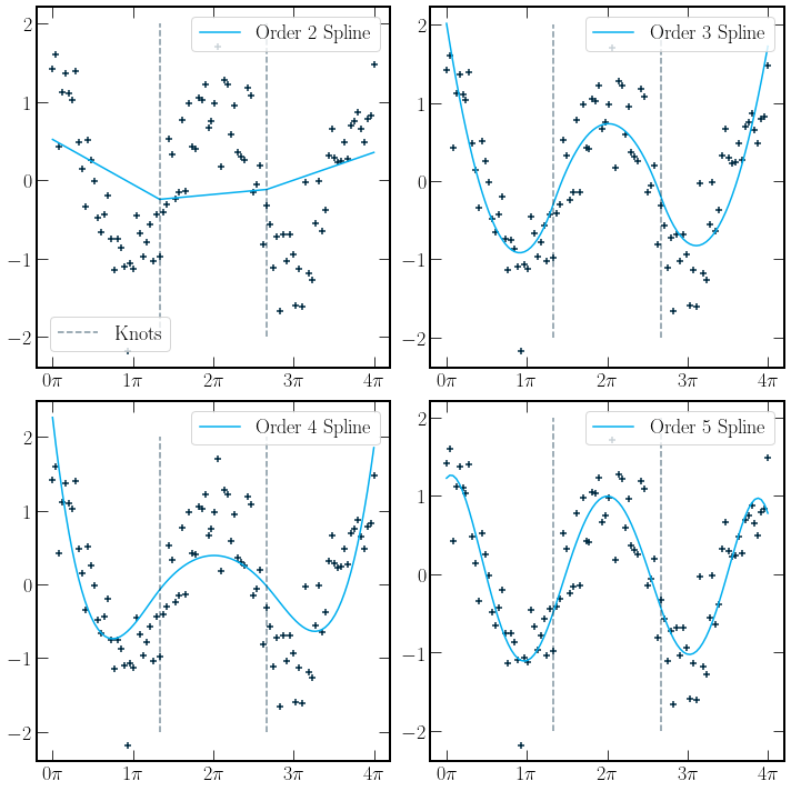
As defined in [HTF09], a spline is piecewise polynomials of order \(m\) with \(m-2\) continuous derivatives. The order-\(m\) spline provides a function, which if defined by the degrees of freedom, has a fixed number of knots, points at which the polynomial changes. In the plot below, spline fits of \(\cos(x)\) with Gaussian noise are plotted. There are two knots for all splines. A dashed grey line indicates the position of the knots. The degrees of freedom for a spline
The \(knots+1\) term comes from the number of separate polynomials. There are 3 constraints per knot; where \(x_k\) is the knot postition, the constraints are as follows
The implementation of the splines below is using a least-squares fitting method. A natural spline extension can be used if the spline fit is used as a predictive model for data in unseen regions. A natural spline has a first-degree polynomial applied to regions outside the training data range. These lines are continuous and have continuous first derivatives.
Typically order-\(4\) splines are used.
fig, ax = plt.subplots(2, 2, figsize=(10, 10))
x = np.linspace(0, np.pi * 4, 100)
xs = np.linspace(0, np.pi * 4, 5)
spline_knots = np.linspace(0, np.pi * 4, 4)[1:-1]
y = np.cos(x) + np.random.randn(100) * 0.4
k = 0
for i in range(2):
    for j in range(2):
        k += 1
        spline = LSQUnivariateSpline(
            x,
            y,
            t=spline_knots,
            k=k,
        )
        ax[i, j].scatter(x, y, color=colours.durham.ink)
        ax[i, j].plot(
            x,
            spline(x),
            label=f"Order {k+1} Spline",
            color=colours.durham.blue,
        )
        ax[i, j].set_xticks(xs)
        ax[i, j].set_xticklabels([f"{int(i/np.pi)}$\pi$" for i in xs])
        ax[i, j].legend(loc="upper right")
        for l in spline_knots:
            line = ax[i, j].plot(
                [l, l],
                [-2, 2],
                color=colours.durham.ink,
                alpha=0.5,
                linestyle="--",
                label="Knot",
            )
fig.legend(line, ["Knots"], bbox_to_anchor=(-0.75, 0.59, 0.98, 0.02))
fig.tight_layout()


