Using Bayesian Inference to Determine \(S\) Left as Work in progress

Bayes’ theorem describes a systematic fashion to update one’s beliefs. It explains how independent evidence updates the probability of a given outcome. Bayesian inference is the process in which data is used as the evidence to update the parameters of a model. Inference in this manner also provides a distribution of likelihoods of the model parameter to be estimated.

The Bayesian framework is structured differently, to classical statistics in that it describes an estimate of a state of knowledge, rather than a relative frequency of outcomes. Bayes’ Rule is given as follows

\[P(A|B) = \frac{P(B|A) P(A)}{P(B)} = \frac{P(B|A) P(A)}{\sum_k P(B|K) P(K)}.\]

\(P(A|B)\) is the probability of \(A\) occurring given \(B\). Where \(A, B\) are random variables with some associated distribution. \(P(A|B)\) can be considered the intersection over a subspace of outcomes and is defined in that manner

\[P(A|B) = \frac{P(A \cap B)}{P(B)}.\]

By noting that \(P(A \cap B) = P(B \cap A)\), one can show Bayes’ rule, which is left as an exercise.

If the two random variables are continuous and share a joint distribution \(f_{A,B}(x,y)\) the Bayes’ rule can be described as follows

\[f_{A|B}(x|y) = \frac{ f_{B|A}(y|x) f_A(x)} {\int_{-\infty}^{\infty} f_{B|A}(y|u) f_A(u) du}\]

This formulation is preferable going forward.

Tip

Basic probability theory is covered well in Mathmatical Methods for Physics and Engineering[RHB02], if this feels unfamiliar.

It might not be apparent how random variables are associated with measurement, however when one takes a measurement this is just sampeling a parent distribution of a random variable. By virtue of sampeling a random variable described by a PDF. The valued of the samples are generally normally distributed, around the mean of the parent distribution, due to the central limit theorem(CLT). However, there are some cases where CLT does not hold, when the parent distribution from which the sample is taken lacks a well-defined mean and standard deviation, or the random variables are not independent. A brief and functional treatment can be found in [HH10].

Bayesian Inference

In the least-squares framework of line fitting a straight line, there is a solution to a set of simultaneous equations which minimizes the squared residuals. The value of these residuals can then be assessed with the \(\chi^2\) metric, which enables one to assign a probability that such a set of residuals occur randomly and thus decide if the model is suitable.

Conversely, the Bayesian framework produces a PDF or PMF of the best-fit parameters.

import pandas as pd
import numpy as np
import matplotlib.pyplot as plt
from dur_utils import colours
from scipy.optimize import curve_fit
from scipy import stats
plt.style.use('../CDS.mplstyle')

On the previous page, 3 \(\textrm{CO}_2\) concentration pathways were determined. The \(\textrm{CO}_2\) concentration for each pathway is denoted as \(C_1, C_2, C_3\) for A1B, A1T and B1, respectively. Each of these concentration random variables is additionally a function of time. The PDF for the prediction at time \(t\) for each scenario is
$\( f_{C_i(t)}(c) = \exp(\frac{(c-\bar{c}(t))^2}{2\cdot \sigma_c(t)^2}), \textrm{for} i = 1, 2, 3. \)\( Where \)\bar{c}(t)\( is the predicted value of concentration at time \)t\(, and \)\sigma_c(t)\( is the unctertainty on the fit at that time. Using the dubious assuption that climate sensitivity \)S\( and concentration \)c$ are independent a joint probability distribution of both quantities can be formed.

Note

The climate sensitivity \(S\) is not the random varuable but a value of the random variable. The capitalisation is kept for consitency with the literature[SWA+20, SGS22] despite it being confusing. The random variable that governs the value of \(s\) is denoted as \(\mathcal{S}\).

Having prevously determined a moving average trend for Temperature, and an associated error, with a function that relates the $\( f_{ T, C_i, \mathcal{S}}(\Delta T, S, c) = f_{T, C_i(t)}(c)f_{\mathcal{S}}, \textrm{for} i = 1, 2, 3. \)\( In order to calculate the rise in temperature given an emmisions pathway the distribuiton of possible temperatures \)\( f_{ T|C_i,\mathcal{S}}(T|S, c) = \)$

xs = np.linspace(-3, 3, 1000)
lam = stats.norm.pdf(xs, loc=-1.3, scale=0.44)
del_f = stats.norm.pdf(xs, loc=4.00, scale=0.3)
xs_2 = np.linspace(-3, 10, 1999)
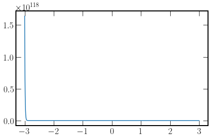
plt.plot(xs, 1.3/del_f)

[<matplotlib.lines.Line2D at 0x7f56a7bb7fa0>]